How the measurement works.
Nyquist gives us the relationship. The engineering challenge is everything that follows: extracting a microvolt-scale random signal from amplifier noise, the calibration signal and electromagnetic interference.
The relation
Thermal agitation of charge carriers in a resistor produces a random voltage across it. The mean-square of that voltage depends on temperature, resistance and the bandwidth over which we observe it, and on nothing else:
Mean square noise voltage equals four times the Boltzmann constant, times thermodynamic temperature, times resistance, times bandwidth.
Rearranged for the quantity we actually want:
Thermodynamic temperature equals mean square noise voltage divided by four times the Boltzmann constant, times resistance, times bandwidth.
Since 2019 the Boltzmann constant has been fixed by definition, not measured, so kB contributes no uncertainty. That leaves three quantities for us to determine: the noise, the resistance and the bandwidth, all of which are electrical. It is why we can make a noise thermometer traceable to electrical standards instead of to a chain of temperature comparisons.
In a real instrument Δf is never a clean rectangular bandwidth, so equation (2) is evaluated as a summation over narrow, individually calibrated frequency bins instead of as a single term.
The ratio, and what it cancels
We do not measure noise in absolute terms. A calibration signal of known magnitude is injected into the system prior to the measurement, and temperature comes from the ratio of the two.
How the two are separated is the part that matters, and it is where this design departs from earlier noise thermometers. Those switch in time: the instrument looks at the sensor, then at a calibration source, and alternates. That only works if the bandwidth of the sensor branch stays put between the two halves of the switch, and over a range of temperatures it does not, because cable capacitance and sensor resistance both move. At that point the result becomes dependent on the very things a noise thermometer exists to be free of. The usual mitigation is to work only at low frequencies, which throttles the available bandwidth and pushes integration times out to minutes or hours.
We do not switch. The calibration signal is a pseudo-random comb of tones, each one centred in an FFT bin so it doesn't leak into its neighbours, and the comb occupies a select number of bins. Johnson noise and calibration signal are therefore present in the same measured output signal at the same time and are separated in the frequency domain: noise power is summed from the bins with no tone in them, and the calibration signal is read from the bins that have one. It's the frequency domain separation approach that makes a 1.2 MHz bandwidth usable, and a wide bandwidth is what makes the measurement fast enough to be useful for real-world industrial applications.
The ratio is what makes the electronics a weak dependency. Amplifier gain appears in both the Johnson noise measurement and the calibration measurement, so it divides out, and the frequency response of almost the entire chain is common to both. A drift that affects both signals equally has no effect on the answer, which is a far more attainable requirement than asking the electronics not to drift at all.
Two chains, one sensor
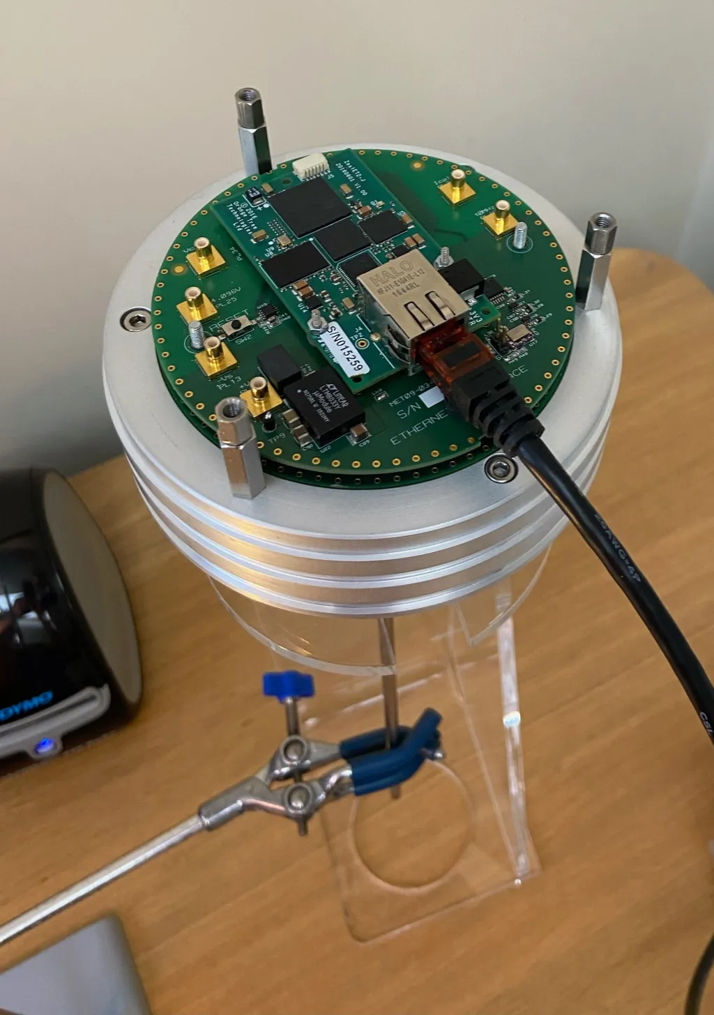
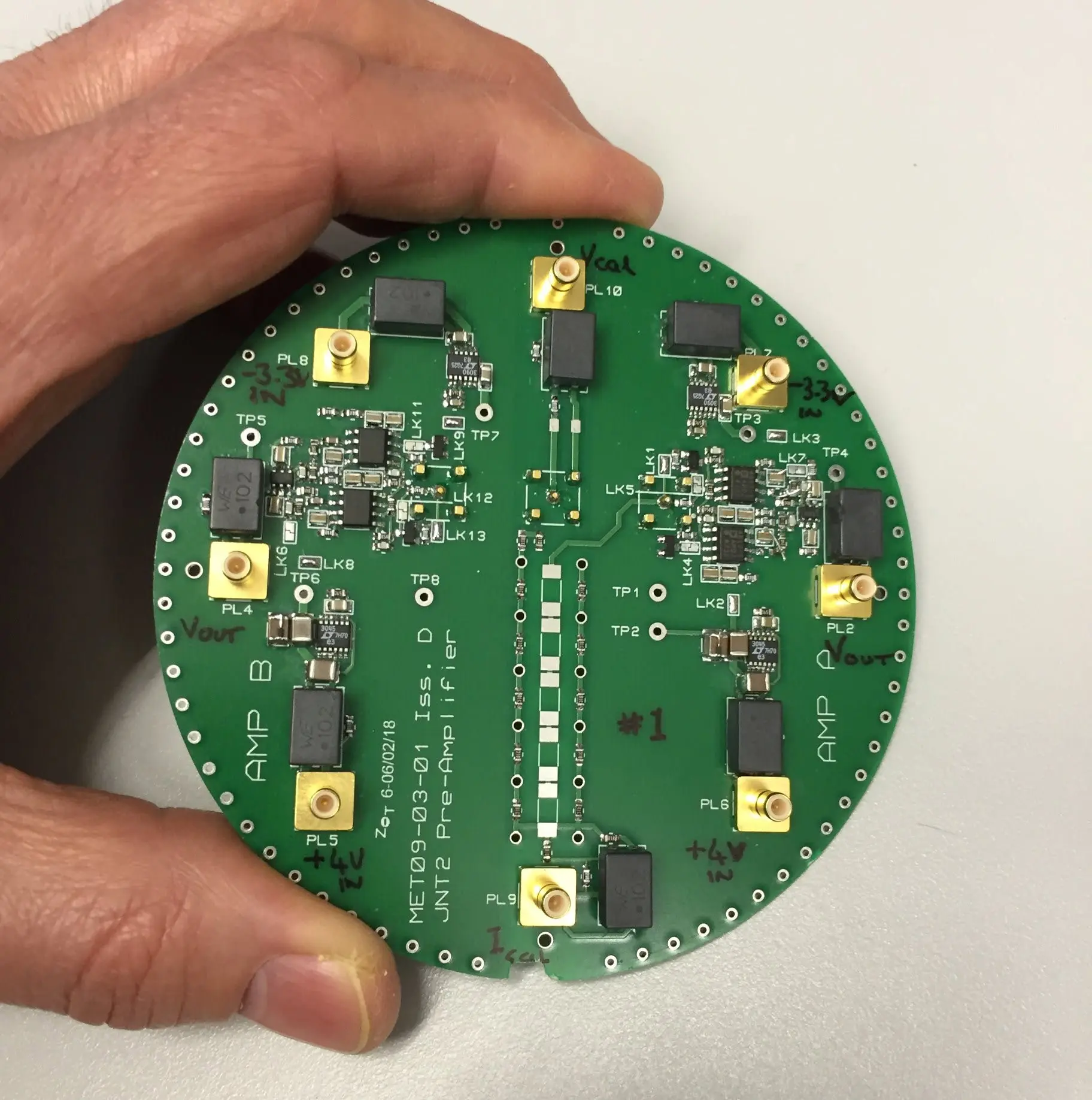
Johnson noise from a 5 kΩ sensor is small enough that the amplifiers reading it generate noise of the same order. Averaging harder does not help, because the amplifier noise averages to its own non-zero value instead of to zero.
Fig. Block diagram of the correlator. Two amplifier chains observe the same sensor. Noise generated independently in either amplifier averages down, while the sensor’s Johnson noise is common to both and remains after cross-correlation.
A calibration signal is injected at the same time as the noise is measured, so both experience the same amplifier gain and frequency response. Temperature is derived from their ratio, making the result largely insensitive to changes in that shared response.
Unlike switching noise thermometers, which measure noise and reference signals at different times, this approach determines noise, calibration and sensor resistance together from the same data.
What sets the uncertainty
Under the operating conditions described here the dominant short-term limit is statistical rather than instrumental. A random signal observed for a finite time gives a finite estimate of its own power, and Rice’s equation puts a floor on how good that estimate can be:
Fractional standard deviation equals one over the square root of bandwidth times observation time.
More bandwidth or more time buys precision, and only as the square root. We work at 1.2 MHz, which is wide for this application, and use a 5 kΩ sensor where earlier work typically used 100 Ω, because a larger resistance produces more signal to begin with.
Wide bandwidth brings its own problem. Sensor resistance combines with cable capacitance to form a low-pass filter, so the signal in each frequency bin falls away at the top of the range while amplifier noise does not. Summing those bins in equally therefore makes the result worse beyond a certain point, and there is an optimum bandwidth to stop at.
Weighting each bin by the inverse of its squared uncertainty removes that ceiling altogether: poor bins contribute in proportion to how little they are worth, so extra bandwidth can only help. On the system in the 2019 paper this cut measurement uncertainty by 28 per cent.
Does it give the right answer?
The test that matters is whether the physics holds somewhere nobody has tuned it. We measure noise power across a range of temperatures, fit a straight line, and project it back to zero power. The intercept ought to land on absolute zero, since at absolute zero there is no thermal agitation and no noise to measure.
For the second-generation prototype the projection lands at −273.415 °C. True absolute zero is −273.15 °C. The residual scatter about the fit is 0.017652 K, so the 0.265 K gap is real and not just noise in the fit. The first prototype missed by 1.36 K under comparable conditions, and this is a projection made from a few hundred degrees away.
The figures on this page are from Developments Towards an Industrial Johnson Noise Thermometer(2019) and from Challenges and solutions in the development of a Johnson noise thermometer (2024). Both, and everything else we have published, are on the publications page.